In the last post I talked about one method to estimate distributional differences from ordinal data, such as those reported by statewide accountability systems. In this post, we’ll put this method to work for the state of California. I’ll show how we can estimate school-level Hispanic/White achievement gaps for every school in the state that reports data on both groups. In California, this means the school must have at least 30 students in each group, for the corresponding grade.

The data

The primary data we’ll be looking at are available here. As I mentioned in the previous post, part of what I think is so cool about this method is that these data are reported across all states, so you could apply this method with any state. I chose California here because I have some experience with their specific data, I’m a west-coaster, and California is more interesting than Oregon (where I live) because they are much more diverse and have areas of dense population.

These data have a number of numeric codes in them that don’t make much sense without the code book, which is available here.

I’m also always interested in geographic variance in social things, including school performance, so I also like to try to grab the longitude and latitude of the schools. That’s available through a separate file, available here. Note that geographic information is available more generally for every public school in the country through the National Center for Education Statistics (NCES) Education Demographic and Geographic Estimates (EDGE) program.

Loading the data

We could, of course, just visit these websites and pull the data down and load it in manually, but that’s no fun. This is R. Let’s do it through code!

The file we want is at http://www3.cde.ca.gov/caasppresearchfiles/2018/sb/sb_ca2018_all_csv_v3.zip. The tricky part is, it’s in a zip file with one other file. One way to handle this is by creating a temporary directory, downloading the zip file there, then unzipping the file and pulling just the data we want out. In our case, the filename is the same as the zip file, but with a .txt extension. I’ll be using the tidyverse later anyway so I’ll do something like this

library(tidyverse)

# create a temporary directory
tmp <- tempdir()

# download the zip file. Call it "file.zip"
download.file("http://www3.cde.ca.gov/caasppresearchfiles/2018/sb/sb_ca2018_all_csv_v3.zip", 
              file.path(tmp, "file.zip"))

# Pull out just the file we want
file <- unzip(file.path(tmp, "file.zip"), files = "sb_ca2018_all_csv_v3.txt")

# Read it into R
d <- read_csv(file) %>%
  janitor::clean_names()
d
## # A tibble: 3,269,730 x 32
##    county_code district_code school_code filler test_year subgroup_id
##    <chr>       <chr>         <chr>       <lgl>      <dbl>       <dbl>
##  1 00          00000         0000000     NA          2018           1
##  2 00          00000         0000000     NA          2018           1
##  3 00          00000         0000000     NA          2018           1
##  4 00          00000         0000000     NA          2018           1
##  5 00          00000         0000000     NA          2018           1
##  6 00          00000         0000000     NA          2018           1
##  7 00          00000         0000000     NA          2018           1
##  8 00          00000         0000000     NA          2018           1
##  9 00          00000         0000000     NA          2018           1
## 10 00          00000         0000000     NA          2018           1
## # … with 3,269,720 more rows, and 26 more variables: test_type <chr>,
## #   total_tested_at_entity_level <dbl>, total_tested_with_scores <dbl>,
## #   grade <dbl>, test_id <dbl>, caaspp_reported_enrollment <dbl>,
## #   students_tested <dbl>, mean_scale_score <dbl>,
## #   percentage_standard_exceeded <dbl>, percentage_standard_met <dbl>,
## #   percentage_standard_met_and_above <dbl>,
## #   percentage_standard_nearly_met <dbl>,
## #   percentage_standard_not_met <dbl>, students_with_scores <dbl>,
## #   area_1_percentage_above_standard <dbl>,
## #   area_1_percentage_near_standard <dbl>,
## #   area_1_percentage_below_standard <dbl>,
## #   area_2_percentage_above_standard <dbl>,
## #   area_2_percentage_near_standard <dbl>,
## #   area_2_percentage_below_standard <dbl>,
## #   area_3_percentage_above_standard <dbl>,
## #   area_3_percentage_near_standard <dbl>,
## #   area_3_percentage_below_standard <dbl>,
## #   area_4_percentage_above_standard <dbl>,
## #   area_4_percentage_near_standard <dbl>,
## #   area_4_percentage_below_standard <dbl>

That gives us the basic file we want, but we don’t know what any of the subgroup IDs represent. To get that, we’ll have to download another datafile. This is another zip file, but note I’m using a slightly different approach below, which I can do because the zip file only contains a single file.

tmp_file <- tempfile()
download.file("http://www3.cde.ca.gov/caasppresearchfiles/2018/sb/subgroups.zip",
              tmp_file)
subgroups <- read_csv(unz(tmp_file, "Subgroups.txt"), 
                      col_names = c("char_num", "subgroup_id", 
                                    "specific_group", "overall_group"))
subgroups
## # A tibble: 47 x 4
##    char_num subgroup_id specific_group                  overall_group      
##    <chr>          <dbl> <chr>                           <chr>              
##  1 001                1 All Students                    All Students       
##  2 003                3 Male                            Gender             
##  3 004                4 Female                          Gender             
##  4 006                6 Fluent English proficient and … English-Language F…
##  5 007                7 Initial fluent English profici… English-Language F…
##  6 008                8 Reclassified fluent English pr… English-Language F…
##  7 028               28 Migrant education               Migrant            
##  8 031               31 Economically disadvantaged      Economic Status    
##  9 074               74 Black or African American       Ethnicity          
## 10 075               75 American Indian or Alaska Nati… Ethnicity          
## # … with 37 more rows

Now we can join these data

d <- left_join(d, subgroups)
d
## # A tibble: 3,269,730 x 35
##    county_code district_code school_code filler test_year subgroup_id
##    <chr>       <chr>         <chr>       <lgl>      <dbl>       <dbl>
##  1 00          00000         0000000     NA          2018           1
##  2 00          00000         0000000     NA          2018           1
##  3 00          00000         0000000     NA          2018           1
##  4 00          00000         0000000     NA          2018           1
##  5 00          00000         0000000     NA          2018           1
##  6 00          00000         0000000     NA          2018           1
##  7 00          00000         0000000     NA          2018           1
##  8 00          00000         0000000     NA          2018           1
##  9 00          00000         0000000     NA          2018           1
## 10 00          00000         0000000     NA          2018           1
## # … with 3,269,720 more rows, and 29 more variables: test_type <chr>,
## #   total_tested_at_entity_level <dbl>, total_tested_with_scores <dbl>,
## #   grade <dbl>, test_id <dbl>, caaspp_reported_enrollment <dbl>,
## #   students_tested <dbl>, mean_scale_score <dbl>,
## #   percentage_standard_exceeded <dbl>, percentage_standard_met <dbl>,
## #   percentage_standard_met_and_above <dbl>,
## #   percentage_standard_nearly_met <dbl>,
## #   percentage_standard_not_met <dbl>, students_with_scores <dbl>,
## #   area_1_percentage_above_standard <dbl>,
## #   area_1_percentage_near_standard <dbl>,
## #   area_1_percentage_below_standard <dbl>,
## #   area_2_percentage_above_standard <dbl>,
## #   area_2_percentage_near_standard <dbl>,
## #   area_2_percentage_below_standard <dbl>,
## #   area_3_percentage_above_standard <dbl>,
## #   area_3_percentage_near_standard <dbl>,
## #   area_3_percentage_below_standard <dbl>,
## #   area_4_percentage_above_standard <dbl>,
## #   area_4_percentage_near_standard <dbl>,
## #   area_4_percentage_below_standard <dbl>, char_num <chr>,
## #   specific_group <chr>, overall_group <chr>

Preparing the data

It’s fairly difficult to see what’s going on here so let’s limit our data to only the things we really care about here. We’ll need the district and school codes, the group variables we just added in, and all the percentage in each category.

d <- d %>%
  select(district_code, school_code, grade, overall_group, specific_group, test_id, 
         percentage_standard_not_met, percentage_standard_nearly_met,
         percentage_standard_met, percentage_standard_exceeded)
d
## # A tibble: 3,269,730 x 10
##    district_code school_code grade overall_group specific_group test_id
##    <chr>         <chr>       <dbl> <chr>         <chr>            <dbl>
##  1 00000         0000000         3 All Students  All Students         1
##  2 00000         0000000         3 All Students  All Students         2
##  3 00000         0000000         4 All Students  All Students         2
##  4 00000         0000000         4 All Students  All Students         1
##  5 00000         0000000         5 All Students  All Students         1
##  6 00000         0000000         5 All Students  All Students         2
##  7 00000         0000000         6 All Students  All Students         2
##  8 00000         0000000         6 All Students  All Students         1
##  9 00000         0000000         7 All Students  All Students         1
## 10 00000         0000000         7 All Students  All Students         2
## # … with 3,269,720 more rows, and 4 more variables:
## #   percentage_standard_not_met <dbl>,
## #   percentage_standard_nearly_met <dbl>, percentage_standard_met <dbl>,
## #   percentage_standard_exceeded <dbl>

As you can see here at the bottom of the page, a test id of 1 means it was English Language Arts, while 2 means Mathematics.

d <- d %>%
  mutate(test_id = ifelse(test_id == 1, "ELA", "Mathematics"))

Now we’ll limit the data to only Hispanic/White students, which is the achievement gap we’ll investigate across schools. I don’t know the specific labels, so I’ll look at these first, then filter accordingly.

d %>%
  filter(overall_group == "Ethnicity") %>%
  count(specific_group)
## # A tibble: 8 x 2
##   specific_group                          n
##   <chr>                               <int>
## 1 American Indian or Alaska Native    36814
## 2 Asian                               66739
## 3 Black or African American           69158
## 4 Filipino                            49836
## 5 Hispanic or Latino                  97442
## 6 Native Hawaiian or Pacific Islander 31804
## 7 Two or more races                   69653
## 8 White                               91827
d <- d %>%
  filter(overall_group == "Ethnicity",
         specific_group == "White" |
           specific_group == "Hispanic or Latino")
d
## # A tibble: 189,269 x 10
##    district_code school_code grade overall_group specific_group test_id
##    <chr>         <chr>       <dbl> <chr>         <chr>          <chr>  
##  1 00000         0000000         3 Ethnicity     Hispanic or L… ELA    
##  2 00000         0000000         3 Ethnicity     Hispanic or L… Mathem…
##  3 00000         0000000         4 Ethnicity     Hispanic or L… Mathem…
##  4 00000         0000000         4 Ethnicity     Hispanic or L… ELA    
##  5 00000         0000000         5 Ethnicity     Hispanic or L… ELA    
##  6 00000         0000000         5 Ethnicity     Hispanic or L… Mathem…
##  7 00000         0000000         6 Ethnicity     Hispanic or L… Mathem…
##  8 00000         0000000         6 Ethnicity     Hispanic or L… ELA    
##  9 00000         0000000         7 Ethnicity     Hispanic or L… ELA    
## 10 00000         0000000         7 Ethnicity     Hispanic or L… Mathem…
## # … with 189,259 more rows, and 4 more variables:
## #   percentage_standard_not_met <dbl>,
## #   percentage_standard_nearly_met <dbl>, percentage_standard_met <dbl>,
## #   percentage_standard_exceeded <dbl>

Notice that the school_code and district_code are both 0 here. This is the code for the overall state, which we probably want to eliminate.

d <- d %>%
  filter(school_code != "0000000")
d
## # A tibble: 160,479 x 10
##    district_code school_code grade overall_group specific_group test_id
##    <chr>         <chr>       <dbl> <chr>         <chr>          <chr>  
##  1 10017         0112607        11 Ethnicity     Hispanic or L… Mathem…
##  2 10017         0112607        11 Ethnicity     Hispanic or L… ELA    
##  3 10017         0112607        13 Ethnicity     Hispanic or L… ELA    
##  4 10017         0112607        13 Ethnicity     Hispanic or L… Mathem…
##  5 10017         0112607        11 Ethnicity     White          Mathem…
##  6 10017         0112607        11 Ethnicity     White          ELA    
##  7 10017         0112607        13 Ethnicity     White          ELA    
##  8 10017         0112607        13 Ethnicity     White          Mathem…
##  9 10017         0123968         3 Ethnicity     Hispanic or L… Mathem…
## 10 10017         0123968         3 Ethnicity     Hispanic or L… ELA    
## # … with 160,469 more rows, and 4 more variables:
## #   percentage_standard_not_met <dbl>,
## #   percentage_standard_nearly_met <dbl>, percentage_standard_met <dbl>,
## #   percentage_standard_exceeded <dbl>

Estimated effect sizes

We now have a pretty basic dataset that we’re ready to use to estimate effect size. If you recall from the previous post, what we need is the cumulate percentage of students in each category, rather than the raw percents. I’m going to do this by first creating a lower category that has zero students in it. I’ll then reshape the data to a long(er) format and calculate the cumulative sum.

Data prep

First, create the lower category

d <- d %>%
  mutate(percentage_standard_low = 0)
d
## # A tibble: 160,479 x 11
##    district_code school_code grade overall_group specific_group test_id
##    <chr>         <chr>       <dbl> <chr>         <chr>          <chr>  
##  1 10017         0112607        11 Ethnicity     Hispanic or L… Mathem…
##  2 10017         0112607        11 Ethnicity     Hispanic or L… ELA    
##  3 10017         0112607        13 Ethnicity     Hispanic or L… ELA    
##  4 10017         0112607        13 Ethnicity     Hispanic or L… Mathem…
##  5 10017         0112607        11 Ethnicity     White          Mathem…
##  6 10017         0112607        11 Ethnicity     White          ELA    
##  7 10017         0112607        13 Ethnicity     White          ELA    
##  8 10017         0112607        13 Ethnicity     White          Mathem…
##  9 10017         0123968         3 Ethnicity     Hispanic or L… Mathem…
## 10 10017         0123968         3 Ethnicity     Hispanic or L… ELA    
## # … with 160,469 more rows, and 5 more variables:
## #   percentage_standard_not_met <dbl>,
## #   percentage_standard_nearly_met <dbl>, percentage_standard_met <dbl>,
## #   percentage_standard_exceeded <dbl>, percentage_standard_low <dbl>

We need this because of the cumulative sum calculation that comes next. First though, let’s reshape the data. After the reshape, I do a tiny bit of cleanup so the category variable doesn’t repeat "percentage_standard_" over and over.

ld <- d %>%
  gather(category, percentage, starts_with("percentage")) %>%
  mutate(category = gsub("percentage_standard_", "", category))

ld
## # A tibble: 802,395 x 8
##    district_code school_code grade overall_group specific_group test_id
##    <chr>         <chr>       <dbl> <chr>         <chr>          <chr>  
##  1 10017         0112607        11 Ethnicity     Hispanic or L… Mathem…
##  2 10017         0112607        11 Ethnicity     Hispanic or L… ELA    
##  3 10017         0112607        13 Ethnicity     Hispanic or L… ELA    
##  4 10017         0112607        13 Ethnicity     Hispanic or L… Mathem…
##  5 10017         0112607        11 Ethnicity     White          Mathem…
##  6 10017         0112607        11 Ethnicity     White          ELA    
##  7 10017         0112607        13 Ethnicity     White          ELA    
##  8 10017         0112607        13 Ethnicity     White          Mathem…
##  9 10017         0123968         3 Ethnicity     Hispanic or L… Mathem…
## 10 10017         0123968         3 Ethnicity     Hispanic or L… ELA    
## # … with 802,385 more rows, and 2 more variables: category <chr>,
## #   percentage <dbl>

Now we need to make sure the categories are ordered in ascending order within a school. The best way to do this, from my perspective, is to transform category into a categorical variable.

unique(ld$category)
## [1] "not_met"    "nearly_met" "met"        "exceeded"   "low"
ld <- ld %>%
  mutate(category = factor(category, 
                           levels = c("low", "not_met", 
                                      "nearly_met", "met", 
                                      "exceeded"))) %>%
  arrange(school_code, grade, specific_group, test_id, category)

ld
## # A tibble: 802,395 x 8
##    district_code school_code grade overall_group specific_group test_id
##    <chr>         <chr>       <dbl> <chr>         <chr>          <chr>  
##  1 65243         0100016         3 Ethnicity     Hispanic or L… ELA    
##  2 65243         0100016         3 Ethnicity     Hispanic or L… ELA    
##  3 65243         0100016         3 Ethnicity     Hispanic or L… ELA    
##  4 65243         0100016         3 Ethnicity     Hispanic or L… ELA    
##  5 65243         0100016         3 Ethnicity     Hispanic or L… ELA    
##  6 65243         0100016         3 Ethnicity     Hispanic or L… Mathem…
##  7 65243         0100016         3 Ethnicity     Hispanic or L… Mathem…
##  8 65243         0100016         3 Ethnicity     Hispanic or L… Mathem…
##  9 65243         0100016         3 Ethnicity     Hispanic or L… Mathem…
## 10 65243         0100016         3 Ethnicity     Hispanic or L… Mathem…
## # … with 802,385 more rows, and 2 more variables: category <fct>,
## #   percentage <dbl>

And now we can calculate the cumulative percentage

ld <- ld %>%
  group_by(school_code, grade, specific_group, test_id) %>%
  mutate(cumm_perc = cumsum(percentage))

ld
## # A tibble: 802,395 x 9
## # Groups:   school_code, grade, specific_group, test_id [160,479]
##    district_code school_code grade overall_group specific_group test_id
##    <chr>         <chr>       <dbl> <chr>         <chr>          <chr>  
##  1 65243         0100016         3 Ethnicity     Hispanic or L… ELA    
##  2 65243         0100016         3 Ethnicity     Hispanic or L… ELA    
##  3 65243         0100016         3 Ethnicity     Hispanic or L… ELA    
##  4 65243         0100016         3 Ethnicity     Hispanic or L… ELA    
##  5 65243         0100016         3 Ethnicity     Hispanic or L… ELA    
##  6 65243         0100016         3 Ethnicity     Hispanic or L… Mathem…
##  7 65243         0100016         3 Ethnicity     Hispanic or L… Mathem…
##  8 65243         0100016         3 Ethnicity     Hispanic or L… Mathem…
##  9 65243         0100016         3 Ethnicity     Hispanic or L… Mathem…
## 10 65243         0100016         3 Ethnicity     Hispanic or L… Mathem…
## # … with 802,385 more rows, and 3 more variables: category <fct>,
## #   percentage <dbl>, cumm_perc <dbl>

And now we’re getting close. We just need a column for each each group. We’ll drop the raw percentage (so rows are uniquely defined) and spread the cumulative sum into to columns according to the specific group

ld %>%
  select(-percentage) %>%
  spread(specific_group, cumm_perc)	
## # A tibble: 429,670 x 8
## # Groups:   school_code, grade, test_id [85,934]
##    district_code school_code grade overall_group test_id category
##    <chr>         <chr>       <dbl> <chr>         <chr>   <fct>   
##  1 10017         0112607        11 Ethnicity     ELA     low     
##  2 10017         0112607        11 Ethnicity     ELA     not_met 
##  3 10017         0112607        11 Ethnicity     ELA     nearly_…
##  4 10017         0112607        11 Ethnicity     ELA     met     
##  5 10017         0112607        11 Ethnicity     ELA     exceeded
##  6 10017         0112607        11 Ethnicity     Mathem… low     
##  7 10017         0112607        11 Ethnicity     Mathem… not_met 
##  8 10017         0112607        11 Ethnicity     Mathem… nearly_…
##  9 10017         0112607        11 Ethnicity     Mathem… met     
## 10 10017         0112607        11 Ethnicity     Mathem… exceeded
## # … with 429,660 more rows, and 2 more variables: `Hispanic or
## #   Latino` <dbl>, White <dbl>

This looks basically correct, but to make it a bit more clear, let’s remove schools that did not report percentages for both groups

ld <- ld %>%
  select(-percentage) %>%
  spread(specific_group, cumm_perc)	%>%
  janitor::clean_names() %>%
  drop_na(hispanic_or_latino, white) %>%
  arrange(school_code, grade, test_id, category) 

ld
## # A tibble: 219,925 x 8
## # Groups:   school_code, grade, test_id [74,545]
##    district_code school_code grade overall_group test_id category
##    <chr>         <chr>       <dbl> <chr>         <chr>   <fct>   
##  1 65243         0100016         3 Ethnicity     ELA     low     
##  2 65243         0100016         3 Ethnicity     Mathem… low     
##  3 65243         0100016         4 Ethnicity     ELA     low     
##  4 65243         0100016         4 Ethnicity     ELA     not_met 
##  5 65243         0100016         4 Ethnicity     ELA     nearly_…
##  6 65243         0100016         4 Ethnicity     ELA     met     
##  7 65243         0100016         4 Ethnicity     ELA     exceeded
##  8 65243         0100016         4 Ethnicity     Mathem… low     
##  9 65243         0100016         4 Ethnicity     Mathem… not_met 
## 10 65243         0100016         4 Ethnicity     Mathem… nearly_…
## # … with 219,915 more rows, and 2 more variables:
## #   hispanic_or_latino <dbl>, white <dbl>

And now we’re very close, but if you look carefully you can see we have one issue remaining - every school has the low category reported for both groups. We need to remove schools that only have the low category reported (because they don’t actually have any real data reported). There’s lots of ways to do this, of course, but a fairly straightforward way is to count the rows within each school/grade/test combination and make sure there are five observations (four categories, plus the low category). Then we’ll select for just those observations.

ld <- ld %>%
  group_by(school_code, grade, test_id) %>%
  mutate(n = n()) %>%
  filter(n == 5) %>%
  select(-n)

ld
## # A tibble: 181,725 x 8
## # Groups:   school_code, grade, test_id [36,345]
##    district_code school_code grade overall_group test_id category
##    <chr>         <chr>       <dbl> <chr>         <chr>   <fct>   
##  1 65243         0100016         4 Ethnicity     ELA     low     
##  2 65243         0100016         4 Ethnicity     ELA     not_met 
##  3 65243         0100016         4 Ethnicity     ELA     nearly_…
##  4 65243         0100016         4 Ethnicity     ELA     met     
##  5 65243         0100016         4 Ethnicity     ELA     exceeded
##  6 65243         0100016         4 Ethnicity     Mathem… low     
##  7 65243         0100016         4 Ethnicity     Mathem… not_met 
##  8 65243         0100016         4 Ethnicity     Mathem… nearly_…
##  9 65243         0100016         4 Ethnicity     Mathem… met     
## 10 65243         0100016         4 Ethnicity     Mathem… exceeded
## # … with 181,715 more rows, and 2 more variables:
## #   hispanic_or_latino <dbl>, white <dbl>

And our data are finally finalized! 🥳

Produce estimates

First, let’s compute the area under the paired curves. To do this, we just use an x/y integration. This will give us one estimate for each school/test/grade combination. I’ll use the {pracma} package again. One small caveat here… to get the correct AUC, the cumulative percentages actually need to be cumulative proportions. We could have done this transformation above in our data prep (and maybe I should have done that) but you can also do it in the integration and it doesn’t change the results at all. We’ll take this approach.

aucs <- ld %>%
  group_by(school_code, grade, test_id) %>%
  summarize(auc = pracma::trapz(hispanic_or_latino / 100, 
                                white / 100)) %>%
  ungroup()

aucs
## # A tibble: 36,345 x 4
##    school_code grade test_id       auc
##    <chr>       <dbl> <chr>       <dbl>
##  1 0100016         4 ELA         0.342
##  2 0100016         4 Mathematics 0.339
##  3 0100016        13 ELA         0.389
##  4 0100016        13 Mathematics 0.420
##  5 0100024         3 ELA         0.429
##  6 0100024         3 Mathematics 0.484
##  7 0100024         4 ELA         0.534
##  8 0100024         4 Mathematics 0.477
##  9 0100024         5 ELA         0.478
## 10 0100024         5 Mathematics 0.445
## # … with 36,335 more rows

As a reminder, these values represent the probability that a randomly selected student from the x axis group, in this case students coded Hispanic/Latino, would score above a randomly selected student from the y axis group, in this case students coded White.

Now, we can transform these values into effect sizes using sqrt(2)*qnorm(auc), where auc represents the values we just calculated.

v <- aucs %>%
  mutate(v = sqrt(2)*qnorm(auc))

v
## # A tibble: 36,345 x 5
##    school_code grade test_id       auc       v
##    <chr>       <dbl> <chr>       <dbl>   <dbl>
##  1 0100016         4 ELA         0.342 -0.577 
##  2 0100016         4 Mathematics 0.339 -0.588 
##  3 0100016        13 ELA         0.389 -0.400 
##  4 0100016        13 Mathematics 0.420 -0.285 
##  5 0100024         3 ELA         0.429 -0.253 
##  6 0100024         3 Mathematics 0.484 -0.0565
##  7 0100024         4 ELA         0.534  0.119 
##  8 0100024         4 Mathematics 0.477 -0.0803
##  9 0100024         5 ELA         0.478 -0.0792
## 10 0100024         5 Mathematics 0.445 -0.195 
## # … with 36,335 more rows

And voilà! We have effect size estimates for every school in California that reported data on both groups.

Quick exploration

This is already a long post, so I’ll keep this brief, but let’s quickly explore the effect size estimates.

First, let’s just look at the distributions by content area.

theme_set(theme_minimal(15))

means <- v %>%
  group_by(test_id) %>%
  summarize(av = mean(v))

ggplot(v, aes(v)) +
  annotate("rect",
           inherit.aes = FALSE,
           ymin = -Inf, 
           ymax = Inf,
           xmin = 0, 
           xmax = Inf,
           fill = "gray40",
           alpha = .8) +
  geom_histogram(fill = "cornflowerblue") +
  geom_vline(aes(xintercept = av), means, size = 1.5, color = "magenta") +
  geom_vline(xintercept = 0, color = "gray80") +
  facet_wrap(~test_id, ncol = 1)

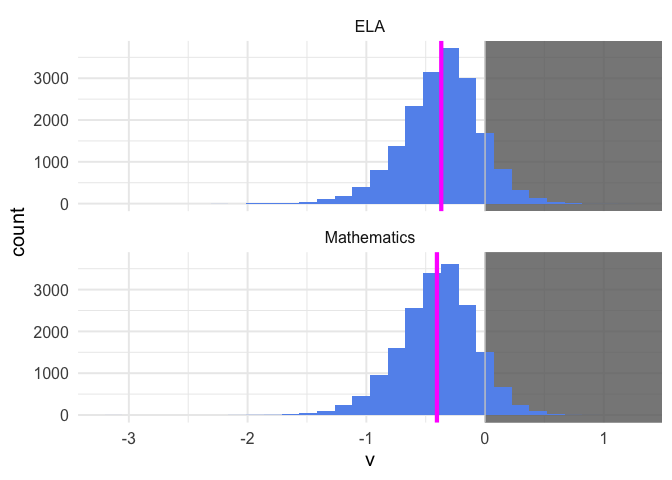
This gives us a quick understanding of the overall distribution. For the vast majority of schools, students coded Hispanic/Latino are scoring, on average, lower than students coded White. But this is not true for all schools. We can also see that these achievement disparities are, on average, slightly larger in Math than in ELA.

Notice, however, that there is considerable variability between schools. What drives this variability? This is currently my primary area of interest.

One more quick exploration, let’s look at the distributions by grade. I’ll use the {ggridges} package to produce distributions by grade.

grade_means <- v %>%
  group_by(grade, test_id) %>%
  summarize(mean = mean(v),
            mean_se = sundry::se(v))

ggplot(v, aes(x = v, y = factor(grade))) +
  ggridges::geom_density_ridges(fill = "cornflowerblue", 
                                alpha = 0.4,
                                color = "white",
                                height = 0.4,
                                scale = 1) +
  geom_segment(aes(x = mean, xend = mean, 
                   y = as.numeric(factor(grade)), 
                   yend = as.numeric(factor(grade)) + 0.7), 
               grade_means,
               color = "gray40",
               lty = "dashed") +
  scale_x_continuous("", limits = c(-1.75, 1)) +
  labs(y  = "Grade",
       title = "Achievement gap effect sizes by grade",
       subtitle = "Effect sizes estimated from ordinal percent proficient data",
       caption = "Data obtained from the California Department of Education website: \n https://caaspp.cde.ca.gov/sb2018/ResearchFileList") +
  facet_wrap(~test_id) 

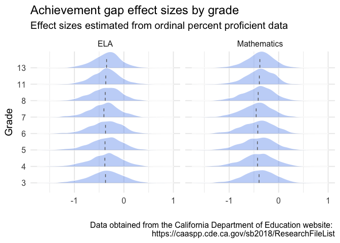
Is there evidence of the achievement gaps growing by grade? Maybe… let’s take a different look.

ggplot(grade_means, aes(grade, mean)) +
  geom_errorbar(aes(ymax = mean + qnorm(0.975)*mean_se,
                    ymin = mean + qnorm(0.025)*mean_se)) +
  geom_point() +
  geom_smooth() +
  facet_wrap(~test_id) +
  scale_x_continuous(breaks = c(3:8, 11, 13))

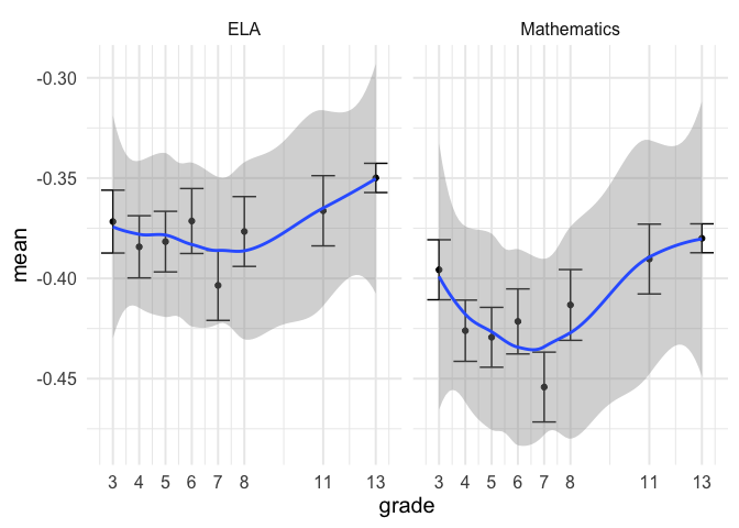
Maybe some, but the evidence is not overwhelmingly strong in this case

Conclusions

This was a long post, but an important one, I think. In the next post, I’ll talk about geographical variation in school-level achievement gaps, which will require linking the schools with data including longitude and latitude, and exploring things like census variables to explore how they may relate to the between-school variability.

Thanks for reading! Please get in touch if you found it interesting, see areas that need correcting, or have follow-up questions.